Building a Model for Retirement Savings in Python
It's easy to find investment advice. It's a little less easy to find good investment advice, but still pretty easy. We are awash in advice on saving for retirement, with hundreds of books and hundreds of thousands of articles written on the subject. It is studied relentlessly, and the general consensus is that it's best to start early, make regular contributions, stick it all in low-fee index funds, and ignore it. I'm not going to dispute that, but I do want to better understand why it works so well. As programmers we don't have to simply take these studies at their word. The data is readily available, and we can explore retirement savings strategies ourselves by writing models in code. Let's take a look at how to build up a model in Python to see how much we can save over the course of a career.
Disclaimer: I am not a financial adviser, so this article should not be taken as financial advice. It is merely an exploration of a model of retirement savings for the purpose of learning and understanding how savings could grow over time.
We'll start with a very simple model to get things started. How about we put in an initial investment of $12,000 at 20 years old and let it grow until retirement at 67. How do we have $12,000 at 20? Maybe it's a gift from a rich aunt and uncle or we saved like crazy during a summer internship between college semesters. Somehow we came up with it. Why $12,000? Because there's 12 months in a year, and that seemed nice. What does it look like after 48 years? Here's a simple exponential model to give us an estimate:
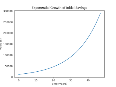
Our little retirement fund reaches nearly $290,000 by the end of our career. That's not too bad considering it was just a single contribution from before we could legally drink, but it's probably not enough to last through retirement, what with inflation and health care and all to consider. What happens if we manage to pull together $12,000 every year and contribute to our nest egg? It's going to be tough in the beginning, but it'll get easier. Plus, those early years are the most important.
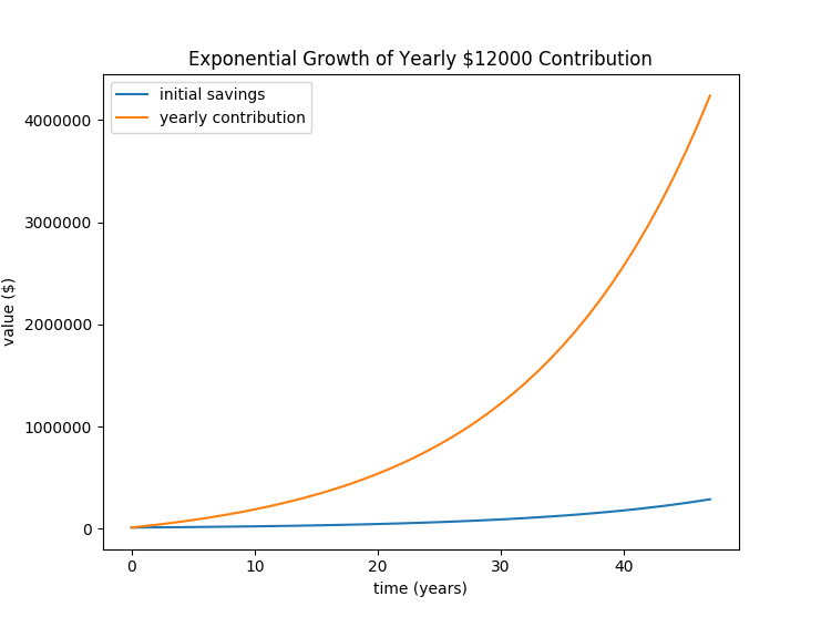
The equation for regular contributions to an exponentially growing investment is a little trickier, but other people have already figured it out so we'll just use what they did. The equation is
value = P*ry + C*(ry - 1)/(r - 1)
Where P is the principle investment, C is the yearly contribution, r is the rate of return in the form of 1.0x for x%, and y is the number of years to invest. Plugging that equation into our Python model gives the following code:
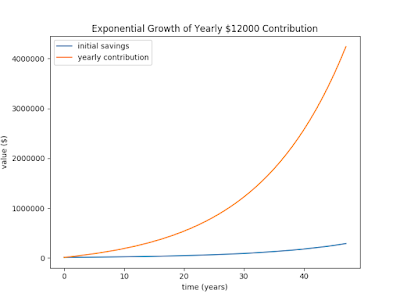
Whoa! After all of that time contributing to saving, we end up with over $4.2 million. That's some serious retirement funds. Now we're really starting to see the power of savings rates with regular contributions. It's not just important to save early, but to save regularly. However, this model is still relatively divorced from the real world. In the real world, we're never going to see a consistent 7% return year after year. Some years it will be less, and some years it will be a lot more. What happens to our plan of consistent yearly contributions when we know that some years we're going to be dropping in a chunk of cash right near the peak of the market?
To answer that question, we can look at historical prices. We used to be able to get a nice, long history of prices for the main market indexes—the Dow Jones, NASDAQ, and S&P500—quite easily from Yahoo and Google APIs, but it seems those sources have been shut down in the last couple years. We can still manually download .csv files of historical prices at finance.yahoo.com, for example the NASDAQ daily prices all the way back to its start in 1971 can be downloaded here. It's not as fun as using an API, but we can easily read this file into our Python script using Pandas read_csv() function, and offset the date so that we can look at years since the beginning of the index:
After the initial investment shares, we can populate a Series that matches the length of our investment period with updated shares as we make additional contributions each year. We loop through the historical prices, and each time we cross into a new year, we add more shares with the next contribution at the price that the index is at that time. Since the first day of trading in the new year doesn't necessarily land on January 2nd, the if condition shows a simple way to detect the first trading day of the new year for each year. Here's how our hypothetical investments did over the last 48 years sitting in the NASDAQ:

Yikes! Not only did we best the simple exponential model, but we blew it away with about $14M in savings by the end. The investments in the fund also never dropped below the conservative 7% estimated rate of return, even during the dotcom crash and the Great Recession. (Okay, it did a little in the beginning, but you can't really see that here.) Why did we do so much better? Partly it's because the NASDAQ has performed better than a 7% return, on average, getting about 9.5% returns over the last 48 years. That doesn't fully explain the better performance, though, because plugging the simple model with 9.5% returns would result in $9.7M by the time we retire.
The other $4.3M in gains comes from all of the contributions that happened while the market was down. This is by far the best time to buy because the market recovers more quickly after it's been down, and the gains of those new contributions are juiced along with the recovering shares that were purchased at higher prices. In the end, the gains are more than they would have been with a smooth rate of return. However, when the market is down, it's also the most difficult time to buy, and it's extremely hard (some say impossible) to predict the market. It's these characteristics that make it so important to stick to the plan of investing early and regularly.
We now have a more accurate hypothetical investment scenario, but we can do even better. So far we've assumed that we're investing the same amount every year. That's a fine goal, but it's going to get really easy to achieve as we get raises over the years. Hopefully we won't be making the same salary at 45 that we were at 25, so let's try to model that by building in a yearly increase to the contributions. Now, we have to make a few assumptions in light of a ton of potential contributing factors. Over the years expenses will likely increase as we buy a house, start a family, and generally start enjoying the fruits of our labor more. Be careful, though. If you find your expenses increasing faster than your salary, it's going to become more difficult to meet your savings goals.
Let's assume that's not the case, and you find a way to moderately increase your expenses over time. Most years it should be fairly straightforward to live on a budget pretty close to the previous year. Sometimes bigger expenses, or step-ups in spending happen, but step-ups in income also happen. Getting married or otherwise becoming a dual-income household is generally a big step-up. Promotions will also give a good boost to income. These positive things combined with a steady budget can result in most of the increased income being available for savings. Since savings is only a percentage of your total income, this means a big increase in savings. For example, suppose you're saving 20% of your income, and you get a 5% raise. If you sock all of that raise into savings, that equates to a 25% increase in savings. Since step-ups like that doesn't happen every year, let's keep things simple and assume a 5% increase in savings every year. That results in the following calculations:
Now we're looking at about $24M available in retirement! This keeps getting better. Another nice thing about this investment is that it doesn't have to end at retirement. There are tons of options for taking out some funds to safely live off of and continue investing the rest, letting it grow further during retirement. Making donations to worthy causes is also a definite possibility here. You know, spread the wealth that you have been so blessed with. Of course, we have many, many years ahead of us before this nest egg becomes a reality, so let's focus on the model we're exploring. We can look at another inaccuracy that's been in the model for a while, namely that we're investing one big chunk of money each year. It should be better to invest smaller amounts more often, so let's split the yearly contribution into bimonthly paycheck contributions, 24 total for each year.

Huh, it's a little more difficult to see any difference with the paycheck contribution approach. This was actually a bit surprising because I expected more of an increase due to investing earlier and more frequently. To see how much of a difference there really is, we can plot the difference between the paycheck contributions and the yearly contributions:

It turns out that we make an extra $1.3M over the full 48 years, but it takes some time to build up and is never more than about 5% of the total investment. The accumulation of exponential gains over the entire investment period is much more important than the small additional gains we get by spreading the yearly contributions over the course of each year. Even so, it's probably best to plug that money into the retirement fund as soon as it's available, just so that it'll be saved instead of spent. The small extra gains to be had from investing it a little bit earlier is a little extra bonus.
One thing we haven't modeled here is what happens if we could optimize our investment performance through buying and selling at opportune times, otherwise known as timing the market. This is a really bad idea for at least three reasons. First—and the most often cited reason—it's extremely difficult to time the market successfully, and do it consistently. The day-to-day movements in the market are so noisy that it's anyone's guess (and it really is a guess) which way the market is going to move at any given time. Even if you have a 50-50 shot of getting it right on any given trade, you're not going to get ahead at all by doing this. More likely, you'll fall behind because of the next reason.
Second, if you're selling a lot, it's probably short sales, and the taxes on those sales are going to erode your realized gains. That means you have to be doing that much better on your returns, just to break even with keeping your money parked in a fund. If the gains are going to be taxed at a marginal rate of 25%, and you're managing to make returns of 11%, then after taxes your gains are actually only 8.25%. That's less than the 9.5% average gains of the NASDAQ. You would actually need to get returns of 12.7% just to break even with leaving your money alone. As your investments grow, it gets even harder to beat the market because the larger gains push you into a higher tax bracket. At the 35% bracket you have to achieve gains of 14.6% just to break even. Granted, you could limit this market timing to tax-advantaged accounts, but that will become a smaller and smaller percentage of your total investments if you keep increasing your contributions. The smaller fraction of tax-advantaged funds will matter less and less over time. Plus, refer back to the first reason, or risk watching your tax-advantaged retirement accounts dwindle instead of grow.
Third, if you stick to index funds, as you should, you are limited in how soon you can sell after buying a fund. Depending on how you're investing, this limit can be 30 to 90 days from your last contribution. This limitation makes timing the market all the more difficult and fraught with risk. But that's a feature, not a bug. It discourages trying to do something you just shouldn't do. If you really want to try being a day trader, you're going to have to go with individual stocks, and that path carries its own set of bigger risks and an even bigger time commitment. Besides, look at those graphs of our investments. Nearly all of the downturns in the market were in the noise, save the dotcom crash and the Great Recession, and the latter doesn't even look like that big of a deal in the graph considering the recovery afterward. The bottom line is, you shouldn't sell. That is, unless you're ready to sell.
The one case where it's probably okay to sell early is if we've already overshot our long-term goals. Take a look back at the last graph. At the peak of the dotcom boom, before the bust, the model is showing investments of nearly $13.7M in the 29th year. If our goal was $10M or less by retirement, then it would be perfectly fine to sell off a significant amount of that position, pay the taxes on the long-term gains, and sink it into a more stable investment for safe-keeping. Or we may even decide to retire early! When the market crashes and the index fund is cheap again, we may even decide to get back in and benefit from the recovery. The point is that selling to get out of the market and then buying later to get back in had nothing to do with trying to predict the dotcom boom and bust. We were simply acting on the fact that our goals were met, and then we saw a prime opportunity that we couldn't pass up. Suffice it to say, these situations don't come up very often. In this 48-year span it only happened once, arguably twice with the housing crash, so it should not be a strategy to depend on happening frequently.
We've learned a great deal from this set of simple models. It's surprising how little code is needed to get a clear picture of some solid investment strategies. It's so obvious that it's great to start early and let the wonders of exponential growth work for you. Investing often—at least once a year—makes a huge difference in the value of your nest egg. Continuing to increase the contributions over time also maximizes your savings potential, and even adds significantly to the accumulated savings in later years. The best part is how easy it is to experiment once we have a working model. We can twiddle with the parameters and see how changes affect the outcome. Through that experimentation, we can get more comfortable with why certain recommendations make good sense, and better understand which investment strategy will help us reach our retirement goals with minimal fuss.
Disclaimer: I am not a financial adviser, so this article should not be taken as financial advice. It is merely an exploration of a model of retirement savings for the purpose of learning and understanding how savings could grow over time.
We'll start with a very simple model to get things started. How about we put in an initial investment of $12,000 at 20 years old and let it grow until retirement at 67. How do we have $12,000 at 20? Maybe it's a gift from a rich aunt and uncle or we saved like crazy during a summer internship between college semesters. Somehow we came up with it. Why $12,000? Because there's 12 months in a year, and that seemed nice. What does it look like after 48 years? Here's a simple exponential model to give us an estimate:
import pandas as pd
import numpy as np
import matplotlib.pyplot as plt

rate = 1.07
years_saving = 48
initial_savings = 12000
model = pd.DataFrame({'t': range(years_saving)})
model['simple_exp'] = [initial_savings*rate**year for year in model.t]

plt.figure()
plt.plot(model.t, model.simple_exp)
plt.title('Exponential Growth of Initial Savings')
plt.xlabel('time (years)')
plt.ylabel('value ($)')

Our little retirement fund reaches nearly $290,000 by the end of our career. That's not too bad considering it was just a single contribution from before we could legally drink, but it's probably not enough to last through retirement, what with inflation and health care and all to consider. What happens if we manage to pull together $12,000 every year and contribute to our nest egg? It's going to be tough in the beginning, but it'll get easier. Plus, those early years are the most important.
The equation for regular contributions to an exponentially growing investment is a little trickier, but other people have already figured it out so we'll just use what they did. The equation is
value = P*ry + C*(ry - 1)/(r - 1)
Where P is the principle investment, C is the yearly contribution, r is the rate of return in the form of 1.0x for x%, and y is the number of years to invest. Plugging that equation into our Python model gives the following code:
yearly_contribution = 12000
model['yearly_invest'] = model['simple_exp'] + [yearly_contribution*(rate**year - 1)/(rate-1) for year in model.t]
plt.plot(model.t, model.yearly_invest)
plt.title('Exponential Growth of Yearly $' + str(yearly_contribution) + ' Contribution')
plt.legend(['initial savings', 'yearly contribution'])
To answer that question, we can look at historical prices. We used to be able to get a nice, long history of prices for the main market indexes—the Dow Jones, NASDAQ, and S&P500—quite easily from Yahoo and Google APIs, but it seems those sources have been shut down in the last couple years. We can still manually download .csv files of historical prices at finance.yahoo.com, for example the NASDAQ daily prices all the way back to its start in 1971 can be downloaded here. It's not as fun as using an API, but we can easily read this file into our Python script using Pandas read_csv() function, and offset the date so that we can look at years since the beginning of the index:
ixic = pd.read_csv('ixic.csv')
ixic['Date'] = pd.to_datetime(ixic['Date'])
ixic['t'] = (ixic.Date - ixic.Date.min()) / np.timedelta64(1, 'Y')

shares = initial_savings / ixic.Close.iloc[0]
share_col = pd.Series(index=ixic.index)
for index, row in ixic.iterrows():
    if row.t >= round(row.t) and ixic.t.iloc[index-1] < round(row.t):
        shares += yearly_contribution / row.Close
    share_col.iloc[index] = shares
ixic['shares'] = share_col
plt.plot(ixic.t, ixic.Close*ixic.shares)
plt.title('Index Fund Performance of Yearly $' + str(yearly_contribution) + ' Contribution')
plt.legend(['initial savings', 'yearly contribution', 'index fund'])
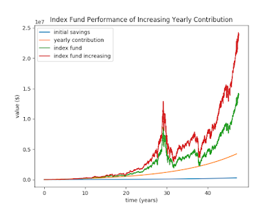
After the initial investment shares, we can populate a Series that matches the length of our investment period with updated shares as we make additional contributions each year. We loop through the historical prices, and each time we cross into a new year, we add more shares with the next contribution at the price that the index is at that time. Since the first day of trading in the new year doesn't necessarily land on January 2nd, the if condition shows a simple way to detect the first trading day of the new year for each year. Here's how our hypothetical investments did over the last 48 years sitting in the NASDAQ:

Yikes! Not only did we best the simple exponential model, but we blew it away with about $14M in savings by the end. The investments in the fund also never dropped below the conservative 7% estimated rate of return, even during the dotcom crash and the Great Recession. (Okay, it did a little in the beginning, but you can't really see that here.) Why did we do so much better? Partly it's because the NASDAQ has performed better than a 7% return, on average, getting about 9.5% returns over the last 48 years. That doesn't fully explain the better performance, though, because plugging the simple model with 9.5% returns would result in $9.7M by the time we retire.
The other $4.3M in gains comes from all of the contributions that happened while the market was down. This is by far the best time to buy because the market recovers more quickly after it's been down, and the gains of those new contributions are juiced along with the recovering shares that were purchased at higher prices. In the end, the gains are more than they would have been with a smooth rate of return. However, when the market is down, it's also the most difficult time to buy, and it's extremely hard (some say impossible) to predict the market. It's these characteristics that make it so important to stick to the plan of investing early and regularly.
We now have a more accurate hypothetical investment scenario, but we can do even better. So far we've assumed that we're investing the same amount every year. That's a fine goal, but it's going to get really easy to achieve as we get raises over the years. Hopefully we won't be making the same salary at 45 that we were at 25, so let's try to model that by building in a yearly increase to the contributions. Now, we have to make a few assumptions in light of a ton of potential contributing factors. Over the years expenses will likely increase as we buy a house, start a family, and generally start enjoying the fruits of our labor more. Be careful, though. If you find your expenses increasing faster than your salary, it's going to become more difficult to meet your savings goals.
Let's assume that's not the case, and you find a way to moderately increase your expenses over time. Most years it should be fairly straightforward to live on a budget pretty close to the previous year. Sometimes bigger expenses, or step-ups in spending happen, but step-ups in income also happen. Getting married or otherwise becoming a dual-income household is generally a big step-up. Promotions will also give a good boost to income. These positive things combined with a steady budget can result in most of the increased income being available for savings. Since savings is only a percentage of your total income, this means a big increase in savings. For example, suppose you're saving 20% of your income, and you get a 5% raise. If you sock all of that raise into savings, that equates to a 25% increase in savings. Since step-ups like that doesn't happen every year, let's keep things simple and assume a 5% increase in savings every year. That results in the following calculations:
shares = initial_savings / ixic.Close.iloc[0]
share_col = pd.Series(index=ixic.index)
for index, row in ixic.iterrows():
    if row.t >= round(row.t) and ixic.t.iloc[index-1] < round(row.t):
        shares += yearly_contribution / row.Close
        yearly_contribution *= 1.05
    share_col.iloc[index] = shares
ixic['shares_inc'] = share_col
plt.plot(ixic.t, ixic.Close*ixic.shares_inc)
plt.title('Index Fund Performance of Increasing Yearly Contribution')
plt.legend(['initial savings', 'yearly contribution', 'index fund', 'index fund increasing'])

Now we're looking at about $24M available in retirement! This keeps getting better. Another nice thing about this investment is that it doesn't have to end at retirement. There are tons of options for taking out some funds to safely live off of and continue investing the rest, letting it grow further during retirement. Making donations to worthy causes is also a definite possibility here. You know, spread the wealth that you have been so blessed with. Of course, we have many, many years ahead of us before this nest egg becomes a reality, so let's focus on the model we're exploring. We can look at another inaccuracy that's been in the model for a while, namely that we're investing one big chunk of money each year. It should be better to invest smaller amounts more often, so let's split the yearly contribution into bimonthly paycheck contributions, 24 total for each year.
payday_contribution = 500
shares = initial_savings / ixic.Close.iloc[0]
share_col = pd.Series(index=ixic.index)
prev_day = ixic.Date.iloc[0].day
for index, row in ixic.iterrows():
    today = ixic.Date.iloc[index-1].day
    if prev_day > 15 and today < 10 or prev_day < 15 and today >= 15:
        shares += payday_contribution / row.Close
    if row.t >= round(row.t) and ixic.t.iloc[index-1] < round(row.t):
        payday_contribution *= 1.05
    share_col.iloc[index] = shares
    prev_day = today
ixic['shares_inc_payday'] = share_col
plt.plot(ixic.t, ixic.Close*ixic.shares_inc_payday)
plt.title('Index Fund Performance of Increasing Paycheck Contribution')
plt.legend(['initial savings', 'yearly contribution', 'index fund', 'index fund increasing', 'index fund payday'])

Huh, it's a little more difficult to see any difference with the paycheck contribution approach. This was actually a bit surprising because I expected more of an increase due to investing earlier and more frequently. To see how much of a difference there really is, we can plot the difference between the paycheck contributions and the yearly contributions:

One thing we haven't modeled here is what happens if we could optimize our investment performance through buying and selling at opportune times, otherwise known as timing the market. This is a really bad idea for at least three reasons. First—and the most often cited reason—it's extremely difficult to time the market successfully, and do it consistently. The day-to-day movements in the market are so noisy that it's anyone's guess (and it really is a guess) which way the market is going to move at any given time. Even if you have a 50-50 shot of getting it right on any given trade, you're not going to get ahead at all by doing this. More likely, you'll fall behind because of the next reason.
Second, if you're selling a lot, it's probably short sales, and the taxes on those sales are going to erode your realized gains. That means you have to be doing that much better on your returns, just to break even with keeping your money parked in a fund. If the gains are going to be taxed at a marginal rate of 25%, and you're managing to make returns of 11%, then after taxes your gains are actually only 8.25%. That's less than the 9.5% average gains of the NASDAQ. You would actually need to get returns of 12.7% just to break even with leaving your money alone. As your investments grow, it gets even harder to beat the market because the larger gains push you into a higher tax bracket. At the 35% bracket you have to achieve gains of 14.6% just to break even. Granted, you could limit this market timing to tax-advantaged accounts, but that will become a smaller and smaller percentage of your total investments if you keep increasing your contributions. The smaller fraction of tax-advantaged funds will matter less and less over time. Plus, refer back to the first reason, or risk watching your tax-advantaged retirement accounts dwindle instead of grow.
Third, if you stick to index funds, as you should, you are limited in how soon you can sell after buying a fund. Depending on how you're investing, this limit can be 30 to 90 days from your last contribution. This limitation makes timing the market all the more difficult and fraught with risk. But that's a feature, not a bug. It discourages trying to do something you just shouldn't do. If you really want to try being a day trader, you're going to have to go with individual stocks, and that path carries its own set of bigger risks and an even bigger time commitment. Besides, look at those graphs of our investments. Nearly all of the downturns in the market were in the noise, save the dotcom crash and the Great Recession, and the latter doesn't even look like that big of a deal in the graph considering the recovery afterward. The bottom line is, you shouldn't sell. That is, unless you're ready to sell.
The one case where it's probably okay to sell early is if we've already overshot our long-term goals. Take a look back at the last graph. At the peak of the dotcom boom, before the bust, the model is showing investments of nearly $13.7M in the 29th year. If our goal was $10M or less by retirement, then it would be perfectly fine to sell off a significant amount of that position, pay the taxes on the long-term gains, and sink it into a more stable investment for safe-keeping. Or we may even decide to retire early! When the market crashes and the index fund is cheap again, we may even decide to get back in and benefit from the recovery. The point is that selling to get out of the market and then buying later to get back in had nothing to do with trying to predict the dotcom boom and bust. We were simply acting on the fact that our goals were met, and then we saw a prime opportunity that we couldn't pass up. Suffice it to say, these situations don't come up very often. In this 48-year span it only happened once, arguably twice with the housing crash, so it should not be a strategy to depend on happening frequently.
We've learned a great deal from this set of simple models. It's surprising how little code is needed to get a clear picture of some solid investment strategies. It's so obvious that it's great to start early and let the wonders of exponential growth work for you. Investing often—at least once a year—makes a huge difference in the value of your nest egg. Continuing to increase the contributions over time also maximizes your savings potential, and even adds significantly to the accumulated savings in later years. The best part is how easy it is to experiment once we have a working model. We can twiddle with the parameters and see how changes affect the outcome. Through that experimentation, we can get more comfortable with why certain recommendations make good sense, and better understand which investment strategy will help us reach our retirement goals with minimal fuss.
0 Response to "Building a Model for Retirement Savings in Python"
Post a Comment