Everyday Statistics for Programmers: Averages and Distributions
Programmers work with lots of data, and when you work with any amount of data, statistics will quickly come into play. A basic working knowledge of statistics is a good tool for any programmer to have in their toolbox, one that you will likely use regularly once you're comfortable with it.
In this mini-series I'll go through some of the statistical tools that I use everyday, what to look for when deciding on which tool to use, and how to avoid mistakes that can mess up your results. I'll start with the basics of the basics—the humble average and a few of the most common distributions.
The average, formally called the mean, is the most fundamental concept in statistics. It's the hammer in the statistical toolbox. The trick is to use it on the right nails. An average is easy to calculate. Given a data set, all you need to do is add up all of the samples and divide by the number of samples in the set. Voila, you have a value that lies in the middle of your data set.
In Ruby you could calculate a mean from an array of values with a method like this:
The average is best used on a data set where the samples are independent, meaning they are not related to each other through some dominant parameter of the system, and they are close together relative to their magnitude. In statistics this is called the deviation from the mean, and I'll get into deviations more in a later post. The important thing to remember is that the smaller the deviation is, the more meaningful the mean is as a representation of the data set. If a certain data set is a set of temperature measurements with an average of 200°C and varies from 199°C to 201°C, the average is going to say a lot more about the temperature of the data than if the measurements varied from 100°C to 300°C.
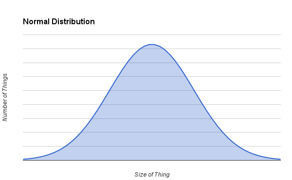
The other important thing to consider when using averages is the distribution of the data. The best case scenario for using averages is if the data has a normal distribution. This type of distribution results from a data set whose samples are clustered around the mean value in a way that's not biased to one side or the other. If you group samples into ranges of values and plot the results as a histogram, you would get something like this for a normal distribution:
You can calculate the histogram bin counts in Ruby with a method like this:
Histograms can tell you a lot about the characteristics of a data set. They will clearly show whether the average is a meaningful representation of the data, how spread out the samples are within the data set, and if there are any peculiarities hidden in the data set. If your data looks like a normal distribution, there are a lot of statistical tools at your disposal for analyzing it.
The mean is also well-defined. It sits right at the peak of the histogram. Half of the samples are larger than the mean, and half of the samples are smaller than the mean. If the histogram is narrow and tall, it shows that the distribution is tight, and a lot of samples are very close to the mean value. The mean is a good value to represent the data set in this case, and its usefulness in predicting the value of future samples with the same characteristics is high.
When you expect your data to have a normal distribution, but it doesn't, it's common for the histogram to show one or more additional peaks. This is called a multimodal distribution, or in the most common case of two peaks, a bimodal distribution. A histogram of such a distribution might look like this:

There are a lot of possibilities here, and most bimodal histograms will not look exactly like this one. The peaks could be further apart, one could be narrower than the other, or one could be taller than the other. In any case, the bimodal nature of the data makes an average less characteristic of the data than normal. Depending on how far apart the peaks are, the mean could merely be shifted from where it should be, or it could fall in an area of the data where there are hardly any data points at all—not a terribly useful place for a mean to be.
What this histogram is telling you is that something is affecting the data in a binary way, meaning that the parameter that is affecting the data is takes on two values. When it's one of the two values, the samples will cluster around one mean, and when it's the other value, the samples will cluster around a different mean. Each value of the parameter will create a separate normal distribution, and the combination of samples at two different values of this unknown parameter creates the bimodal distribution. In fact, I created the above graph by adding two normal distributions together with two different means.
If you have data with a bimodal distribution, you can approach it in a variety of ways. Normally, the first thing you want to do, if you don't know already, is figure out what is causing the distribution to split. Did conditions change while taking the data? Is there some unknown variable that you should filter on to split the data into two sets? What can you control better when taking the data? Can this unknown variable take on more than two values, and if so, does that have a deterministic effect on the data? Can you control this variable to optimize things in the system? Exploring and answering these questions can lead to important new insights into the behavior of the system you're analyzing.
Once you know more about what's causing the bimodal distribution, you can decide whether you want to eliminate the cause or use it to enhance the system. That will depend on whether this variable has a desirable effect on the system or not. In either case, bimodal distributions shouldn't be feared. You can learn a lot about a system by exploring why such a distribution exists.
One last very common distribution is a power-law distribution, also known as a Pareto distribution. This kind of distribution shows up all the time when measuring things with a hard one-sided limit, and it generally looks like this:

The initial sharp decline and then gradual sloping fade away of the curve gives the right side of this distribution the name "the long tail." Many times there is no bounded upper limit to how large whatever is being measured can get. Some examples of things that follow a power-law distribution include people's incomes, internet response times, and user scores on websites like Stackoverflow.com. Some distributions, like people's incomes, have a peak that occurs above zero, but they all exhibit the long tail.
The long tail does some interesting things to the mean of the distribution. A few extremely large data points can pull the mean towards them, giving the mean a potentially large bias. Instead of having a mean being balanced between two equal halves of the distribution, you'll have a distribution with less data points that are larger than the mean and more points that are smaller than the mean.
If you are interested in the halfway point of the distribution, you'll have to calculate the median instead. The median is the value that occurs at the exact halfway point when the samples are sorted. The distance between the median and the mean can be used as a measure of how skewed the distribution is towards the tail.
While the mean is not a very useful parameter of a power-law distribution, knowing that you have such a distribution can guide your use of the data. If the goal is to minimize whatever you're measuring—internet response times is a good example—it can be quite fruitful to target the large outliers to see if they can be eliminated. If those super long response times can't be reduced, they will be a constant drag on the average response time, no matter how much you reduce the faster response times. If instead your goal is to increase the metric, finding some way to affect a large portion of the samples that are below the median will have a correspondingly large effect on the average.
To wrap up, the three main types of distributions that tend to show up when analyzing data are the normal, bimodal, and power-law distributions. When starting to analyze a new data set, it's best to figure out what kind of distribution you're dealing with before diving into more complicated statistical analysis. If the data follows a normal distribution, the mean can be used to talk about what a typical sample is like. With other distributions, you should be much more careful when talking about the average value of the data. That's enough for today. Now that the basics are covered, next time I'll get into standard deviations and confidence.
In this mini-series I'll go through some of the statistical tools that I use everyday, what to look for when deciding on which tool to use, and how to avoid mistakes that can mess up your results. I'll start with the basics of the basics—the humble average and a few of the most common distributions.
The average, formally called the mean, is the most fundamental concept in statistics. It's the hammer in the statistical toolbox. The trick is to use it on the right nails. An average is easy to calculate. Given a data set, all you need to do is add up all of the samples and divide by the number of samples in the set. Voila, you have a value that lies in the middle of your data set.
In Ruby you could calculate a mean from an array of values with a method like this:
module Statistics
  def mean(data)
    data.inject(0.0) { |sum, val| sum + val } / data.size
  end
endThe average is best used on a data set where the samples are independent, meaning they are not related to each other through some dominant parameter of the system, and they are close together relative to their magnitude. In statistics this is called the deviation from the mean, and I'll get into deviations more in a later post. The important thing to remember is that the smaller the deviation is, the more meaningful the mean is as a representation of the data set. If a certain data set is a set of temperature measurements with an average of 200°C and varies from 199°C to 201°C, the average is going to say a lot more about the temperature of the data than if the measurements varied from 100°C to 300°C.
The other important thing to consider when using averages is the distribution of the data. The best case scenario for using averages is if the data has a normal distribution. This type of distribution results from a data set whose samples are clustered around the mean value in a way that's not biased to one side or the other. If you group samples into ranges of values and plot the results as a histogram, you would get something like this for a normal distribution:
You can calculate the histogram bin counts in Ruby with a method like this:
module Statistics
  def self.histogram(data, bins, min_val=nil, max_val=nil)
    min_val ||= data.min
    max_val ||= data.max
    step = (max_val - min_val) / bins.to_f
    counts = [0]*bins
    data.each do |value|
      bin = [((value-min_val)/step).floor, bins - 1].min
      counts[bin] += 1
    end
    counts
  end
endHistograms can tell you a lot about the characteristics of a data set. They will clearly show whether the average is a meaningful representation of the data, how spread out the samples are within the data set, and if there are any peculiarities hidden in the data set. If your data looks like a normal distribution, there are a lot of statistical tools at your disposal for analyzing it.
The mean is also well-defined. It sits right at the peak of the histogram. Half of the samples are larger than the mean, and half of the samples are smaller than the mean. If the histogram is narrow and tall, it shows that the distribution is tight, and a lot of samples are very close to the mean value. The mean is a good value to represent the data set in this case, and its usefulness in predicting the value of future samples with the same characteristics is high.
When you expect your data to have a normal distribution, but it doesn't, it's common for the histogram to show one or more additional peaks. This is called a multimodal distribution, or in the most common case of two peaks, a bimodal distribution. A histogram of such a distribution might look like this:
There are a lot of possibilities here, and most bimodal histograms will not look exactly like this one. The peaks could be further apart, one could be narrower than the other, or one could be taller than the other. In any case, the bimodal nature of the data makes an average less characteristic of the data than normal. Depending on how far apart the peaks are, the mean could merely be shifted from where it should be, or it could fall in an area of the data where there are hardly any data points at all—not a terribly useful place for a mean to be.
What this histogram is telling you is that something is affecting the data in a binary way, meaning that the parameter that is affecting the data is takes on two values. When it's one of the two values, the samples will cluster around one mean, and when it's the other value, the samples will cluster around a different mean. Each value of the parameter will create a separate normal distribution, and the combination of samples at two different values of this unknown parameter creates the bimodal distribution. In fact, I created the above graph by adding two normal distributions together with two different means.
If you have data with a bimodal distribution, you can approach it in a variety of ways. Normally, the first thing you want to do, if you don't know already, is figure out what is causing the distribution to split. Did conditions change while taking the data? Is there some unknown variable that you should filter on to split the data into two sets? What can you control better when taking the data? Can this unknown variable take on more than two values, and if so, does that have a deterministic effect on the data? Can you control this variable to optimize things in the system? Exploring and answering these questions can lead to important new insights into the behavior of the system you're analyzing.
Once you know more about what's causing the bimodal distribution, you can decide whether you want to eliminate the cause or use it to enhance the system. That will depend on whether this variable has a desirable effect on the system or not. In either case, bimodal distributions shouldn't be feared. You can learn a lot about a system by exploring why such a distribution exists.
One last very common distribution is a power-law distribution, also known as a Pareto distribution. This kind of distribution shows up all the time when measuring things with a hard one-sided limit, and it generally looks like this:
The initial sharp decline and then gradual sloping fade away of the curve gives the right side of this distribution the name "the long tail." Many times there is no bounded upper limit to how large whatever is being measured can get. Some examples of things that follow a power-law distribution include people's incomes, internet response times, and user scores on websites like Stackoverflow.com. Some distributions, like people's incomes, have a peak that occurs above zero, but they all exhibit the long tail.
The long tail does some interesting things to the mean of the distribution. A few extremely large data points can pull the mean towards them, giving the mean a potentially large bias. Instead of having a mean being balanced between two equal halves of the distribution, you'll have a distribution with less data points that are larger than the mean and more points that are smaller than the mean.
If you are interested in the halfway point of the distribution, you'll have to calculate the median instead. The median is the value that occurs at the exact halfway point when the samples are sorted. The distance between the median and the mean can be used as a measure of how skewed the distribution is towards the tail.
While the mean is not a very useful parameter of a power-law distribution, knowing that you have such a distribution can guide your use of the data. If the goal is to minimize whatever you're measuring—internet response times is a good example—it can be quite fruitful to target the large outliers to see if they can be eliminated. If those super long response times can't be reduced, they will be a constant drag on the average response time, no matter how much you reduce the faster response times. If instead your goal is to increase the metric, finding some way to affect a large portion of the samples that are below the median will have a correspondingly large effect on the average.
To wrap up, the three main types of distributions that tend to show up when analyzing data are the normal, bimodal, and power-law distributions. When starting to analyze a new data set, it's best to figure out what kind of distribution you're dealing with before diving into more complicated statistical analysis. If the data follows a normal distribution, the mean can be used to talk about what a typical sample is like. With other distributions, you should be much more careful when talking about the average value of the data. That's enough for today. Now that the basics are covered, next time I'll get into standard deviations and confidence.
0 Response to "Everyday Statistics for Programmers: Averages and Distributions"
Post a Comment