Everyday Statistics for Programmers: Standard Deviations and Confidence
Last week I laid some groundwork for understanding statistics that you can use everyday. Calculating averages and looking at histograms to get an idea of what kind of data you're dealing with is a great first step in statistical analysis. But there are so many more tools available, especially if your data approximates a normal distribution. A couple of those tools are standard deviations and confidence intervals, and they can help you understand the characteristics of your data in more detail.
It's important to remember that these tools work best when used with data sets that have a normal distribution because the equations of the tools describe properties of the normal distribution. The more your data set's distribution differs from a normal distribution, the less descriptive power these tools will have for your data. With that cautionary note out of the way, let's tackle some statistics.
The standard deviation is a measure of how tightly clustered a data set's samples are around the mean. As more samples occur closer to the mean, the standard deviation goes down. If the samples are more spread out, it goes up. The following graph shows what different normal distributions look like with standard deviations of 1, 2, and 0.5:

The above description of standard deviation nearly tells you how to calculate it. You could memorize a formula, but it's good to understand the reasoning behind the tools you use so that you can derive the formula even if you can't remember it. Here's how I would build up the formula for the standard deviation:
At this point you may be asking why we squared the differences and then took the square root of the variance. Why not just take the absolute value of the differences, find the mean, and call it a day? If you think of every sample as a separate dimension of the variance of the data set, then the difference between the mean and each sample can be considered a vector. The way to find the magnitude of a vector is to calculate the square root of the sum of squares of its elements. That's exactly what the standard deviation formula does.
Now that we have figured out how to calculate the standard deviation of a data set, here's what it would look like in Ruby code:
The mean and standard deviation together are very useful for describing data. If you talk about a data set as the mean plus or minus two standard deviations, you get a pretty good idea of the range of values for a particular variable. For example, if you have a set of temperature data with a mean of 25°C and a standard deviation of 2.5°C, you can say that the data has a value of 25±5°C to show that it represents a range of temperature values that mostly vary between 20°C and 30°C.
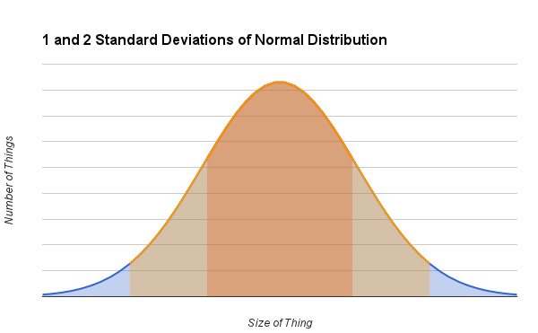
Using two standard deviations to represent the range of a data set is fairly typical. Two standard deviations happens to cover slightly more than 95% of a data set with a normal distribution, so it's a good way of showing the typical values that the data are expected to take on. One standard deviation covers about 68% of the normal distribution. Three standard deviations cover nearly the entire normal distribution at 99.7%, so it's correspondingly much less likely to see values outside of three standard deviations. The following graph shows what one and two standard deviations look like on the normal distribution:
Another way to use the standard deviation is to describe how confident we are that the mean of the data lies within a certain range of values. Our confidence will also depend on the size of the data set for which we're calculating the mean. This makes sense. If you have 10,000 samples you should be much more confident of where the average is than if you only have 100 samples to work with. The range of values that should include the mean to a certain confidence level is referred to as a confidence interval.
To calculate a confidence interval, all you have to do is find the number of standard deviations that will give you the desired confidence level and divide by the square root of the number of samples in the data set. A 95% confidence level is commonly used, and that corresponds to 2 standard deviations (well, actually 1.96, but 2 is easier to remember for quick and dirty calculations). Adding to our example Ruby code, we can use the following method for calculating a 95% confidence interval:
We should be careful here not to say that there is a 95% chance that the average temperature lies in the calculated range. It's a subtle distinction from the above phrasing, but it's wrong. It also starts down a slippery slope to making dubious claims about the data.
The problem with saying there's a 95% chance is that you are no longer talking about confidence. You are talking about probability, and saying there is a probability that the average temperature is within that range is not correct. The average may or may not be within this confidence interval, but it is a definite value, whether you know it or not. That means once you have a confidence interval, the true mean is either in it or not. There is no probability involved. If you don't know what the true mean is—and many times you can't know because you're only sampling from a larger population—then you have a confidence level that the mean is within the range that you calculated.
There are many more details and subtleties contained within these concepts, but with these basics you can find a lot of practical applications of standard deviations and confidence intervals when working with data. Standard deviations help describe the spread of data that follows a normal distribution, and confidence intervals give you a sense of how meaningful the mean of a data set is. Both of these tools can give you a deeper understanding of the data you're analyzing.
Next week we'll take a look at significance, a tool that goes further into figuring out if your data is really saying what you think it is.
It's important to remember that these tools work best when used with data sets that have a normal distribution because the equations of the tools describe properties of the normal distribution. The more your data set's distribution differs from a normal distribution, the less descriptive power these tools will have for your data. With that cautionary note out of the way, let's tackle some statistics.
The standard deviation is a measure of how tightly clustered a data set's samples are around the mean. As more samples occur closer to the mean, the standard deviation goes down. If the samples are more spread out, it goes up. The following graph shows what different normal distributions look like with standard deviations of 1, 2, and 0.5:
The above description of standard deviation nearly tells you how to calculate it. You could memorize a formula, but it's good to understand the reasoning behind the tools you use so that you can derive the formula even if you can't remember it. Here's how I would build up the formula for the standard deviation:
- From the description, we know that we need to start with the mean of the data set and then find the distance (i.e. difference) of every sample from the mean.
- We don't care if the difference is positive or negative, so we'll square each difference to remove its sign.
- We're looking for a general value representing the spread of the data, so we can calculate the average of all of the squared differences to come to a single representative value of the data. This value, as calculated so far, is actually called the variance of the data.
- We're almost there. The only problem is that the units of the variance are squared. To get back to the sample units, take the square root of the variance.
At this point you may be asking why we squared the differences and then took the square root of the variance. Why not just take the absolute value of the differences, find the mean, and call it a day? If you think of every sample as a separate dimension of the variance of the data set, then the difference between the mean and each sample can be considered a vector. The way to find the magnitude of a vector is to calculate the square root of the sum of squares of its elements. That's exactly what the standard deviation formula does.
Now that we have figured out how to calculate the standard deviation of a data set, here's what it would look like in Ruby code:
module Statistics
  def self.sum(data)
    data.inject(0.0) { |s, val| s + val }
  end

  def self.mean(data)
    sum(data) / data.size
  end

  def self.variance(data)
    mu = mean data
    squared_diff = data.map { |val| (mu - val) ** 2 }
    mean squared_diff
  end

  def self.stdev(data)
    Math.sqrt variance(data)
  end
endThe mean and standard deviation together are very useful for describing data. If you talk about a data set as the mean plus or minus two standard deviations, you get a pretty good idea of the range of values for a particular variable. For example, if you have a set of temperature data with a mean of 25°C and a standard deviation of 2.5°C, you can say that the data has a value of 25±5°C to show that it represents a range of temperature values that mostly vary between 20°C and 30°C.
Using two standard deviations to represent the range of a data set is fairly typical. Two standard deviations happens to cover slightly more than 95% of a data set with a normal distribution, so it's a good way of showing the typical values that the data are expected to take on. One standard deviation covers about 68% of the normal distribution. Three standard deviations cover nearly the entire normal distribution at 99.7%, so it's correspondingly much less likely to see values outside of three standard deviations. The following graph shows what one and two standard deviations look like on the normal distribution:
Another way to use the standard deviation is to describe how confident we are that the mean of the data lies within a certain range of values. Our confidence will also depend on the size of the data set for which we're calculating the mean. This makes sense. If you have 10,000 samples you should be much more confident of where the average is than if you only have 100 samples to work with. The range of values that should include the mean to a certain confidence level is referred to as a confidence interval.
To calculate a confidence interval, all you have to do is find the number of standard deviations that will give you the desired confidence level and divide by the square root of the number of samples in the data set. A 95% confidence level is commonly used, and that corresponds to 2 standard deviations (well, actually 1.96, but 2 is easier to remember for quick and dirty calculations). Adding to our example Ruby code, we can use the following method for calculating a 95% confidence interval:
module Statistics
  def self.confidence_interval_95(data)
    mu = mean data
    delta = 1.96 * stdev(data) / Math.sqrt(data.size)
    [mu - delta, mu + delta]
  end
endWe should be careful here not to say that there is a 95% chance that the average temperature lies in the calculated range. It's a subtle distinction from the above phrasing, but it's wrong. It also starts down a slippery slope to making dubious claims about the data.
The problem with saying there's a 95% chance is that you are no longer talking about confidence. You are talking about probability, and saying there is a probability that the average temperature is within that range is not correct. The average may or may not be within this confidence interval, but it is a definite value, whether you know it or not. That means once you have a confidence interval, the true mean is either in it or not. There is no probability involved. If you don't know what the true mean is—and many times you can't know because you're only sampling from a larger population—then you have a confidence level that the mean is within the range that you calculated.
There are many more details and subtleties contained within these concepts, but with these basics you can find a lot of practical applications of standard deviations and confidence intervals when working with data. Standard deviations help describe the spread of data that follows a normal distribution, and confidence intervals give you a sense of how meaningful the mean of a data set is. Both of these tools can give you a deeper understanding of the data you're analyzing.
Next week we'll take a look at significance, a tool that goes further into figuring out if your data is really saying what you think it is.
0 Response to "Everyday Statistics for Programmers: Standard Deviations and Confidence"
Post a Comment